Install TensorFlow on Apple Silicon Macs

First we install TensorFlow on the M1, then we run a small functional test and finally we do a benchmark comparison with an AWS system.

The installation of TensorFlow is very simple#

First, install an ARM version of Python. Recommended (as of 03.2021) is Python 3.8. Version 3.9 is currently not compatible. You can simply install PyCharm (free community version for M1 Mac). This will give you a fully functional Python installation.

Once you have installed Python, do the following#

Open a terminal on your Mac and copy the following line of code into it. This will download TensorFlow and install it in a folder of your choice. Alternatively you can select the default folder.

/bin/bash -c "$(curl -fsS https://raw.githubusercontent.com/apple/tensorflow_macos/master/scripts/download_and_install.sh)"

Default-Folder: /Users/customer/tensorflow_macos_venv/

You should get the following message afterwards:

TensorFlow and TensorFlow Addons with ML Compute for macOS 11.0 successfully installed.

The next step is to activate your newly created Virtual Environment. Copy the following command into your terminal:

. tensorflow_macos_venv/bin/activate`

Important: Do not forget the period at the beginning!

Your prompt should have changed like this now:

(tensorflow_macos_venv) customer@oh-xxx-xxx-xxx-xxx

Now you can start python and import TensorFlow with import tensorflow as tf. You can see with the command tf.__version__ if everything worked. Your output should look like this now:

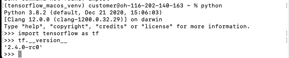
With this the basic installation of TensorFlow is already done.

More information about the current state of the TensorFlow release and which features are not yet supported can be found on the repository page: https://github.com/tensorflow/tensorflow

A small basic application to see if everything works properly#

For this we use the MNIST dataset with handwritten numbers. One of the most popular DataSets to enter the world of Machine Learning and Image Classification. The corresponding Jupyter notebook with more details is available here:

https://www.tensorflow.org/tutorials/quickstart/beginner

import tensorflow as tf

mnist = tf.keras.datasets.mnist

(x_train, y_train), (x_test, y_test) = mnist.load_data()
x_train, x_test = x_train / 255.0, x_test / 255.0`

model = tf.keras.models.Sequential([ 
 tf.keras.layers.Flatten(input_shape=(28, 28)),
 tf.keras.layers.Dense(128, activation='relu'),
 tf.keras.layers.Dropout(0.2),
 tf.keras.layers.Dense(10)
 ])`
predictions = model(x_train[:1]).numpy()
print(predictions)

Output: (The output values may differ slightly, since the forecast is of course recreated)

[[ 0.50077856 0.46635205 -0.04764563 0.0613101 -1.2088307 0.2828893
0.37654606 -0.20382181 -0.903594 0.04570436]]

loss_fn = tf.keras.losses.SparseCategoricalCrossentropy(from_logits=True)
print(loss_fn(y_train[:1], predictions).numpy())Output:

Output:

2.0790117

model.compile(optimizer='adam',
 loss=loss_fn,
 metrics=['accuracy'])

print(model.fit(x_train, y_train, epochs=5))

You may get a warning message:

tensorflow/core/platform/profile_utils/cpu_utils.cc:126] Failed to get CPU frequency: 0 Hz

TensorFlow for Apple Silicon is currently (March 2021) still in an alpha version and certainly still contains one or two bugs. However, most of it already works very well and very fast. Often more than 3s are needed per epoch with Intel CPU and GPU.

Output:

Epoch 1/5
1875/1875 [==============================] - 1s 357us/step - loss: 0.5219 - accuracy: 0.8408

Epoch 2/5
1875/1875 [==============================] - 1s 358us/step - loss: 0.2014 - accuracy: 0.9393

Epoch 3/5
1875/1875 [==============================] - 1s 360us/step - loss: 0.1568 - accuracy: 0.9521

Epoch 4/5
1875/1875 [==============================] - 1s 361us/step - loss: 0.1345 - accuracy: 0.9591

Epoch 5/5
1875/1875 [==============================] - 1s 355us/step - loss: 0.1196 - accuracy: 0.9638
<tensorflow.python.keras.callbacks.History object at 0x10f663670>

print(model.evaluate(x_test, y_test, verbose=2))

Output:

313/313 - 0s - loss: 2.4059 - accuracy: 0.0905

[2.405911684036255, 0.09049999713897705]

probability_model = tf.keras.Sequential([
 model,
 tf.keras.layers.Softmax()
])

print(probability_model(x_test[:5]))

Output:

tf.Tensor(

[[0.05310559 0.05768739 0.14392214 0.04889955 0.11977675 0.17591962
0.08728485 0.12659737 0.06151325 0.12529361]

[0.04891613 0.02110806 0.16333279 0.20522392 0.10033478 0.05052991
0.11514534 0.06312083 0.12917142 0.1031168 ]

[0.09449682 0.06958783 0.1278147 0.086374 0.09083354 0.13517839
0.08620356 0.09317197 0.09092354 0.1254157 ]

[0.06520557 0.04453962 0.1340602 0.08413237 0.07909293 0.10583147
0.1035168 0.06752329 0.14527227 0.17082547]

[0.04817105 0.05779015 0.13250412 0.08222131 0.09708948 0.14379048
0.05646132 0.1505455 0.12961316 0.10181346]],
shape=(5, 10), dtype=float32)

Perfect!

The Benchmark#

Now it gets really exciting! How does our small model with 8 GB RAM perform in the benchmark?

We take as comparison the benchmark of https://www.neuraldesigner.com/blog/training-speed-comparison-gpu-approximation

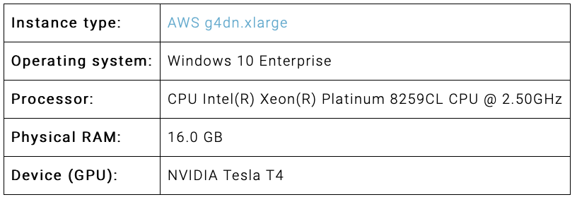
The data from the comparison computer at AWS:

Theoretically, our little Mac should score much worse, since this is a real ML monster, we are curious!

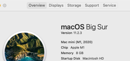
The specs of our Mac Mini M1:

To run the example Pandas and Numpyy must be installed.

The installation of pandas fails if you try to do it via pip install pandas. For a successful installation numpy cython is necessary. Here are the instructions:

pip install --upgrade pip
pip install numpy cython
git clone https://github.com/pandas-dev/pandas.git
cd pandas
python3 setup.py install

The data used is downloadable from the link above and here is the code used, identical to the benchmark:

import tensorflow as tf
import pandas as pd
import time
import numpy as np

# read data float32
start_time = time.time()
filename = ""/Users/customer/Documents/R_new.csv
df_test = pd.read_csv(filename, nrows=100)
float_cols = [c for c in df_test if df_test[c].dtype == "float64"]
float32_cols = {c: np.float32 for c in float_cols}
data = pd.read_csv(filename, engine='c', dtype=float32_cols)
print("Loading time: ", round(time.time() - start_time), " seconds")

x = data.iloc[:, :-1].values
y = data.iloc[:, [-1]].values

initializer = tf.keras.initializers.RandomUniform(minval=-1., maxval=1.)

# build model
model = tf.keras.models.Sequential([tf.keras.layers.Dense(1000,
 activation='tanh',
 kernel_initializer=initializer,
 bias_initializer=initializer),
 tf.keras.layers.Dense(1,
 activation='linear',
 kernel_initializer=initializer,
 bias_initializer=initializer)])

# compile model
model.compile(optimizer='adam', loss='mean_squared_error')

# train model
start_time = time.time()
history = model.fit(x, y, batch_size=1000, epochs=1000)
print("Training time: ", round(time.time() - start_time), " seconds")

First, the results of the AWS Windows PC:

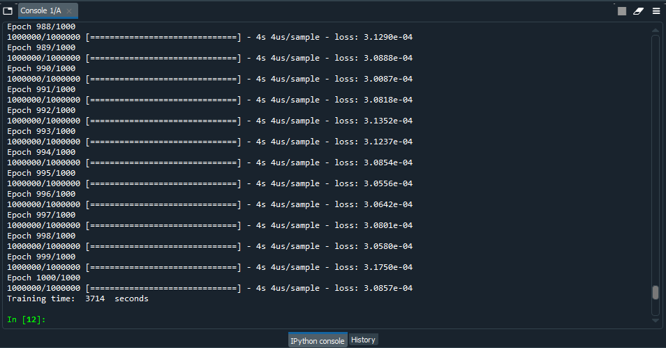
Training time at 1000 epochs was 3714 seconds with an error of 0.0003857 and an average CPU usage of 45%. That's pretty fast!

Now let's give our little Mac Mini a traning:

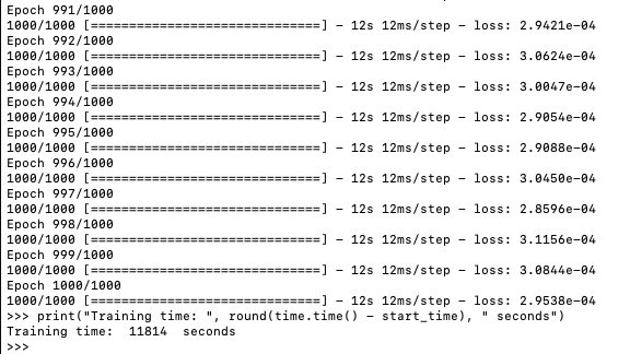
For its specifications, the result is not bad, but I actually expected more from the new chip. Training time at 1000 epochs was 11814 seconds. Apparently there is still some need for optimization as far as large trainig sets are concerned. The same experience was also made in this blog: https://medium.com/analytics-vidhya/m1-mac-mini-scores-higher-than-my-nvidia-rtx-2080ti-in-tensorflow-speed-test-9f3db2b02d74

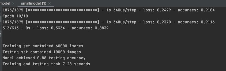
Then let's try the small training set from the blog above:

#import libraries
import tensorflow as tf
import time

#download fashion mnist dataset
fashion_mnist = tf.keras.datasets.fashion_mnist
(train_images, train_labels), (test_images, test_labels) = fashion_mnist.load_data()

train_set_count = len(train_labels)
test_set_count = len(test_labels)

#setup start time
t0 = time.time()

#normalize images
train_images = train_images / 255.0
test_images = test_images / 255.0

#create ML model
model = tf.keras.Sequential([
 tf.keras.layers.Flatten(input_shape=(28, 28)),
 tf.keras.layers.Dense(128, activation='relu'),
 tf.keras.layers.Dense(10)
])

#compile ML model
model.compile(optimizer='adam',
 loss=tf.keras.losses.SparseCategoricalCrossentropy(from_logits=True),
 metrics=['accuracy'])

#train ML model
model.fit(train_images, train_labels, epochs=10)

#evaluate ML model on test set
test_loss, test_acc = model.evaluate(test_images, test_labels, verbose=2)

#setup stop time
t1 = time.time()
total_time = t1-t0

#print results
print('\n')
print(f'Training set contained {train_set_count} images')
print(f'Testing set contained {test_set_count} images')
print(f'Model achieved {test_acc:.2f} testing accuracy')
print(f'Training and testing took {total_time:.2f} seconds')

The result is similar to the blog post, a bit slower because I had a few other applications open:

These values are quite respectable and TensorFlow on ARM is only in the early stages. I am very confident that the performance will improve significantly. Especially for large training sets. And very important: The power consumption and heat generation is minimal! This is a huge advantage for the environment and not least for the wallet!